There will probably be a function to create a map in one run in the next major version of {DatawRappr}. In the meantime, I wrote this tutorial:

There are three map types in Datawrapper: locator, symbol and choropleth. I’m trying to explain in short, how you can use DatawRappr to create a map programmatically for symbols and choropleths. And as an add-on: How to create a tooltip using {DatawRappr}.

Why exclude Locator-maps? They are a little tricky and probably not so heavily automated compared to choropleths and symbols. That’s why I decided place them a little lower on my priority list and keep them out here. There is a tutorial on Locator-maps with the API by Datawrapper using curl.

The basic steps are always the same:

Create a new chart with chart-type map.
Upload your data to this chart/map with the required columns (IDs or Lat/Long-coordinates).
Edit the chart to select the matching for the columns.
Publish the chart.

If you want to update the data, you will only need steps 2 and 4.

Create a Choropleth map

Create a new chart

You can use this code to create a new chart and save the chart to your current environment. You don’t have to save it. You will just need the chart-id later.

new_choropleth_chart <- dw_create_chart(
  title = "This is a automated choropleth map", 
  type = "d3-maps-choropleth"
  )
#> New chart's id: E4ytb

Upload data to the chart

We will now upload some data to our newly created map. Beforehand, we have to decide on an basemap and a key that maps the data to the chart.

Select the right map

Datawrapper provides an API-endpoint with their basemaps, which you might curl

curl --request GET \
  --url https://api.datawrapper.de/plugin/basemaps

Or you can use the built-in dataframe in DatawRappr:

head(dw_basemaps)
#> # A tibble: 6 × 6
#>   id          level  slug   value           label             description       
#>   <chr>       <chr>  <chr>  <chr>           <chr>             <chr>             
#> 1 world-2019  World  world  DW_NAME         Name              The three-letter …
#> 2 world-2019  World  world  NAME_SHORT      Name (short)      The three-letter …
#> 3 world-2019  World  world  DW_STATE_CODE   ISO-Code          The written name …
#> 4 world-2019  World  world  GERMAN_NAME_NEW Name (German)     The written name …
#> 5 world-2019  World  world  GERMAN_NAME     Name old (German) The written name …
#> 6 africa-2020 Africa africa DW_NAME         Name              The three-letter …

First, you have to decide, which map to use. It is identified by the id-column.

You can use dplyr’s View() to get an interactive table. Or you might want to filter using grepl()

dw_basemaps %>% 
  filter(grepl("us-nyc", id))
#> # A tibble: 12 × 6
#>    id                        level       slug        value  label   description 
#>    <chr>                     <chr>       <chr>       <chr>  <chr>   <chr>       
#>  1 us-nyc-boros              USA » New … usa-new-yo… BoroN… Boroug… "Name of th…
#>  2 us-nyc-censustracts       USA » New … usa-new-yo… BoroC… BoroCT… ""          
#>  3 us-nyc-censustracts       USA » New … usa-new-yo… geoid  GEOID … ""          
#>  4 us-nyc-citycouncils       USA » New … usa-new-yo… CounD… Counci… ""          
#>  5 us-nyc-communitydistricts USA » New … usa-new-yo… BoroCD Boro C… ""          
#>  6 us-nyc-hoods              USA » New … usa-new-yo… NTANa… NTA Na… ""          
#>  7 us-nyc-hoods              USA » New … usa-new-yo… NTACo… NTA Co… ""          
#>  8 us-nyc-policeprecincts    USA » New … usa-new-yo… Preci… Precin… ""          
#>  9 us-nyc-schooldistricts    USA » New … usa-new-yo… Schoo… School… ""          
#> 10 us-nyc-uhf                USA » New … usa-new-yo… uhfco… Code    "Name of th…
#> 11 us-nyc-uhf                USA » New … usa-new-yo… uhf_n… Name    "Name of th…
#> 12 us-nyc-zipcodes           USA » New … usa-new-yo… ZIPCO… ZIP co… ""

Select the right key

In a second step, you have to choose a key for the map, which is identified in value. label and description provide some more details about it.

The key is the variable that binds the data to the map.

dw_basemaps %>% 
  filter(grepl("germany-nuts3", id))
#> # A tibble: 2 × 6
#>   id            level                  slug               value     label description
#>   <chr>         <chr>                  <chr>              <chr>     <chr> <chr>      
#> 1 germany-nuts3 Germany » NUTS3 (2016) germany-nuts3-2016 NUTS_NAME Name  The writte…
#> 2 germany-nuts3 Germany » NUTS3 (2016) germany-nuts3-2016 NUTS_ID   Code  code / desc

In this example the basemap germany-nuts3 offers two key-options: NUTS_ID and NUTS_NAME. If you already have one of these options in your dataset, select the right one.

Otherwise, you will have to wrangle the data anyway.

Getting Country IDs

You can easily transform country names in various formats and languages with the {countrycode}-package. In most cases you won’t need a manual translation table. The package is available via CRAN or Github.

After installation, simply add a column with something like countrycode::countrycode(sourcevar = SOURCE VARIABLE, origin = "country.name.de", destination = "iso3c") to your dataframe.

Just in case you need it: You can retrieve the expected keys for a basemap by calling this API-endpoint. Simply enter the id of the basemap and the value of the key:

curl --request GET \
  --url https://api.datawrapper.de/plugin/basemaps/ID/VALUE

you could also use the {jsonlite}-package for this task:

library(jsonlite)

r <- fromJSON("https://api.datawrapper.de/plugin/basemaps/germany-states/name")
r$data$values
#>  [1] "Nordrhein-Westfalen"    "Baden-Württemberg"      "Hessen"                
#>  [4] "Bremen"                 "Niedersachsen"          "Thüringen"             
#>  [7] "Hamburg"                "Schleswig-Holstein"     "Rheinland-Pfalz"       
#> [10] "Saarland"               "Bayern"                 "Berlin"                
#> [13] "Sachsen-Anhalt"         "Sachsen"                "Brandenburg"           
#> [16] "Mecklenburg-Vorpommern"

Upload the data

We are using a simple dataset for German States here as an example: It contains the share of foreign population per German federal state (source: Federal Statistical Office Germany (Destatis)).

df_foreign_pop <- read.csv("data/foreign_pop.csv", stringsAsFactors = FALSE)

str(df_foreign_pop)
#> 'data.frame':    16 obs. of  2 variables:
#>  $ state                   : chr  "Baden-Württemberg" "Bayern" "Berlin" "Brandenburg" ...
#>  $ share_foreign_population: num  15.5 13.2 18.5 4.7 18.1 16.4 16.2 4.5 9.4 13.3 ...

You can simply upload the data as you would do with any other {DatawRappr}-chart.

dw_data_to_chart(df_foreign_pop, chart_id = new_choropleth_chart)
#> Warning in if (format == "csv") {: Bedingung hat Länge > 1 und nur das erste
#> Element wird benutzt
#> Data in E4ytb successfully updated.

Set the keys in the metadata

The metadata of a chart gives us the full flexibility to change what we want to change. In this case, we have to set the axes. A chart in Datawrapper returned as a JSON-Object, which contains differents sublevels. One of those is called metadata and contains the relevant keys:

"metadata": {
      "axes": {
          "keys": "KEY FROM DATA",
          "values": "VALUE FROM DATA"
      },
      "visualize": {
          "basemap": "ID of the basemap",
          "map-key-attr": "VALUE of the map key"
      }
}

In our example from above, we are using the names of the German federal states as the IDs. We will therefore use the basemap germany-states with the value name. name consists of the keys that are already present in our dataset in the state-column. So we don’t need any transformation here. We just need to tell Datawrapper which column to use.

dw_edit_chart(new_choropleth_chart, 
              axes = list(
                keys = "state", 
                values = "share_foreign_population"
                ), 
              visualize = list(
                basemap = "germany-states", 
                "map-key-attr" = "name"
                )
              )
#> Chart E4ytb succesfully updated.

At that point, you might want to switch to Datawrapper’s UI to make the final adjustments to the legend before publishing. But: You could do them via dw_edit_chart as well. It’s probably just not that much fun.

Publish the chart

This is probably the easiest part:

dw_publish_chart(new_choropleth_chart)
#> Chart E4ytb published!
#> ### Responsive iFrame-code: ###
#> <iframe title="This is a automated choropleth map" aria-label="Karte" id="datawrapper-chart-E4ytb" src="https://datawrapper.dwcdn.net/E4ytb/1/" scrolling="no" frameborder="0" style="width: 0; min-width: 100% !important; border: none;" height="580"></iframe><script type="text/javascript">!function(){"use strict";window.addEventListener("message",(function(e){if(void 0!==e.data["datawrapper-height"]){var t=document.querySelectorAll("iframe");for(var a in e.data["datawrapper-height"])for(var r=0;r<t.length;r++){if(t[r].contentWindow===e.source)t[r].style.height=e.data["datawrapper-height"][a]+"px"}}}))}();
#> </script>
#> 
#> ### Chart-URL:###
#> https://datawrapper.dwcdn.net/E4ytb/1/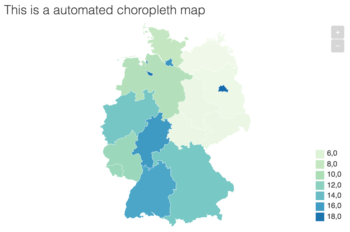

Screenshot of the choropleth map

Create a Symbol map

A symbol map maps a certain value to a geographic location. We will use predefined coordinates here. Datawrapper’s user interface allows geocoding of adresses.

The workflow is pretty similar to the choropleth map. The main difference: We will use Latitude and Longitude coordinates, instead of the key.

Create a new chart

You can use this code to create a new chart and save the chart to your current environment. You don’t have to save it. You will just need the chart-id later.

new_symbol_chart <- dw_create_chart(
  title = "This is a automated symbol map", 
  type = "d3-maps-symbols"
  )
#> New chart's id: PGgcj

Upload data to the chart

We will now upload some data to our newly created map. Beforehand, we have to decide on an basemap.

Select the right map

Datawrapper provides an API-endpoint with their basemaps, which you might curl

curl --request GET \
  --url https://api.datawrapper.de/plugin/basemaps

Or you can use the built-in dataframe in {DatawRappr}:

head(dw_basemaps)
#> # A tibble: 6 × 6
#>   id          level  slug   value           label             description       
#>   <chr>       <chr>  <chr>  <chr>           <chr>             <chr>             
#> 1 world-2019  World  world  DW_NAME         Name              The three-letter …
#> 2 world-2019  World  world  NAME_SHORT      Name (short)      The three-letter …
#> 3 world-2019  World  world  DW_STATE_CODE   ISO-Code          The written name …
#> 4 world-2019  World  world  GERMAN_NAME_NEW Name (German)     The written name …
#> 5 world-2019  World  world  GERMAN_NAME     Name old (German) The written name …
#> 6 africa-2020 Africa africa DW_NAME         Name              The three-letter …

First, you have to decide, which map to use. It is identified by the id-column.

You can use dplyr’s View() to get an interactive table. Or you might want to filter using grepl()

dw_basemaps %>% 
  filter(grepl("us-nyc", id))
#> # A tibble: 12 × 6
#>    id                        level       slug        value  label   description 
#>    <chr>                     <chr>       <chr>       <chr>  <chr>   <chr>       
#>  1 us-nyc-boros              USA » New … usa-new-yo… BoroN… Boroug… "Name of th…
#>  2 us-nyc-censustracts       USA » New … usa-new-yo… BoroC… BoroCT… ""          
#>  3 us-nyc-censustracts       USA » New … usa-new-yo… geoid  GEOID … ""          
#>  4 us-nyc-citycouncils       USA » New … usa-new-yo… CounD… Counci… ""          
#>  5 us-nyc-communitydistricts USA » New … usa-new-yo… BoroCD Boro C… ""          
#>  6 us-nyc-hoods              USA » New … usa-new-yo… NTANa… NTA Na… ""          
#>  7 us-nyc-hoods              USA » New … usa-new-yo… NTACo… NTA Co… ""          
#>  8 us-nyc-policeprecincts    USA » New … usa-new-yo… Preci… Precin… ""          
#>  9 us-nyc-schooldistricts    USA » New … usa-new-yo… Schoo… School… ""          
#> 10 us-nyc-uhf                USA » New … usa-new-yo… uhfco… Code    "Name of th…
#> 11 us-nyc-uhf                USA » New … usa-new-yo… uhf_n… Name    "Name of th…
#> 12 us-nyc-zipcodes           USA » New … usa-new-yo… ZIPCO… ZIP co… ""

Upload the data

We are using a simple dataset for German States here as an example: It contains the share of foreign population per German federal state (source: Federal Statistical Office Germany (Destatis)).

df_foreign_pop_symbol <- read.csv("data/foreign_pop_symbol.csv", stringsAsFactors = FALSE)

str(df_foreign_pop_symbol)
#> 'data.frame':    16 obs. of  4 variables:
#>  $ Lat                     : num  48.6 48.9 52.5 52.8 53.1 ...
#>  $ Lon                     : num  9.19 11.4 13.39 13.25 8.81 ...
#>  $ name                    : chr  "Baden-Württemberg" "Bayern" "Berlin" "Brandenburg" ...
#>  $ share_foreign_population: num  15.5 13.2 18.5 4.7 18.1 16.4 16.2 4.5 9.4 13.3 ...

The data is already geocoded into the Lat and Lon-columns. They are required for the symbol map.

Geocoding Adresses

There are loads of resources on how to geocode places with R. For example, you might want to check out the {ggmap}-package. Unfortunately geocoding with Google does require an API-Key.

For open alternatives you might have a look at hrbrmstr’s {nominatim} or the geocode_OSM()-function in {tmaptools}.

With Lat and Lon-columns set, you can simply upload the data as you would do with any other {DatawRappr}-chart.

dw_data_to_chart(df_foreign_pop_symbol, chart_id = new_symbol_chart)
#> Warning in if (format == "csv") {: Bedingung hat Länge > 1 und nur das erste
#> Element wird benutzt
#> Data in PGgcj successfully updated.

Set the keys in the metadata

"metadata": {
        "axes": {
            "lat": "Lat-Col",
            "lon": "Lon-Col",
            "area": "Value-Col",
            "values": "Value-Col"
        },
      "visualize": {
          "basemap": "world-2019"
      }
}

In our example from above, we are using the names of the German federal states as the IDs. We will therefore use the basemap germany-states. We just need to tell Datawrapper which basemap and columns to use for the mapping. Further options in axes would be:

area: for the area/size of the symbol
value: for the color of the symbol

dw_edit_chart(new_symbol_chart, 
              axes = list(
                lat = "Lat", 
                lon = "Lon",
                area = "share_foreign_population"
                ), 
              visualize = list(
                basemap = "germany-states"
                )
              )
#> Chart PGgcj succesfully updated.

Publish the chart

This is probably the easiest part:

dw_publish_chart(new_symbol_chart)
#> Chart PGgcj published!
#> ### Responsive iFrame-code: ###
#> <iframe title="This is a automated symbol map" aria-label="Karte" id="datawrapper-chart-PGgcj" src="https://datawrapper.dwcdn.net/PGgcj/1/" scrolling="no" frameborder="0" style="width: 0; min-width: 100% !important; border: none;" height="580"></iframe><script type="text/javascript">!function(){"use strict";window.addEventListener("message",(function(e){if(void 0!==e.data["datawrapper-height"]){var t=document.querySelectorAll("iframe");for(var a in e.data["datawrapper-height"])for(var r=0;r<t.length;r++){if(t[r].contentWindow===e.source)t[r].style.height=e.data["datawrapper-height"][a]+"px"}}}))}();
#> </script>
#> 
#> ### Chart-URL:###
#> https://datawrapper.dwcdn.net/PGgcj/1/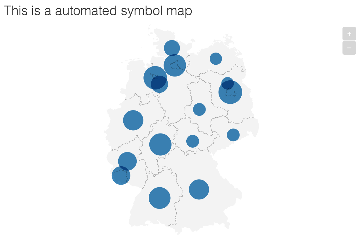

Screenshot of the symbol map

Including tooltips

Including a tooltip is a task that is not only useful for maps, but also for scatterplots. The way to change them via tha API are pretty easy. Just use the visualize-argument in dw_edit_chart() and add a list which includes another list called tooltip.

tooltip has three different keys:

body: which is the body text of the tooltip. Add double brackets ton include a variable: {{ variable }}.
title: is the title of the tooltip. It may also contain a variable with double brackets.
fields: is a list that contains the mapping between the chart data and the variables in the tooltips. You have to include each variable here that is used in the tooltip double brackets in the format: "variable in tooltip" = "variable in data". You may (although it makes things more complicated) map variables to different names, as shown below where "name" = "b".

dw_edit_chart(CHART_ID, visualize = list(
  tooltip = list(
    body = "{{ name }} has value {{ a }}.",
    title = "{{ name }}",
    fields = list(
      "name" = "b",
      "a" = "a"
    )
    )))

Create a Map

Create a Choropleth map

Create a new chart

Upload data to the chart

Select the right map

Select the right key

Upload the data

Set the keys in the metadata

Publish the chart

Create a Symbol map

Create a new chart

Upload data to the chart

Select the right map

Upload the data

Set the keys in the metadata

Publish the chart

Including tooltips